- Blog
Time-series analysis: why causality is the only way


Introduction
Elisa is absent-mindedly glancing through the Research Spotlights column of her favorite eco-blog when a graph grabs her attention:
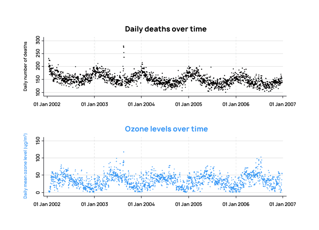
The graph reveals an interesting pattern: the peaks in ozone levels coincide with drops in human deaths, right when summer comes.
Does this mean that ozone helps reduce deaths? Or is it the summer season that is responsible? How can an analyst determine which patterns correspond to causal relationships and which are just correlations?
Discovering causal mechanisms is an integral part of decision-making. By understanding which variables have the capacity to affect others, we can predict how an intervention will impact a system. In this case, reducing the consumption of ozone-depleting substances will probably not immediately reduce the death rate, despite the apparent correlation in our data.
Challenges of determining causality in time series
What makes a time series unique is that the data in it are temporally related. Imagine, for example, what would happen if you randomly permuted the frames in a video — it wouldn’t make much sense because the temporal order matters. In contrast, when statistical analyses are performed on tabular data, the assumption is generally made that the observations are independent and identically distributed: as with the throw of a dice, your expectation of future events does not depend on past ones.
In our example, the ozone level (let’s call it O^3) and the number of deaths (let’s call this variable D) are both time series measured daily for a duration of five years. A common tool to detect correlation in this case is the Poisson regression model. It can tell us whether there exists a linear relationship between O^3 and D (D=x1 O^3 + x2) and with how much certainty our data follow this relationship. The result of this test agrees with what we can see in the graph: high ozone levels correlate with low death rate with high certainty.
However, applying a test on the raw measurements of a time series can lead to wrong conclusions. There are several traps that can completely derail a conclusion:
Long-term trends and seasonality
If we look at the graph, it’s clear that ozone levels peak in the summer, whereas deaths peak in the winter. This is a constant pattern that repeats every year. That means that could be a seasonal effect which is driving both deaths and ozone levels. If that’s the case, how can we remove seasonality from the equation?
In order to answer these questions, we need to go beyond an analysis of the short-term variations. Yes, it’s true that over the course of a given year ozone levels are higher when deaths are lower, but we could also look at the problem on a year-over-year basis, aggregating the number of deaths and the ozone levels over an entire year, and potentially over different cities.
When doing this exercise, we reach the opposite conclusion: higher levels of ozone are indeed associated with higher deaths. The negative correlation was hidden because we failed to take into this seasonal effect, which confounded ozone levels and deaths.
This is a classical example of Simpson’s paradox, which can only be solved if we fully understand the causal structure underlying the data. Simpson’s paradoxes appear in many business settings and lead machines to make the opposite decisions, as they can’t tell a spurious correlation from a true causal effect.
Confounders
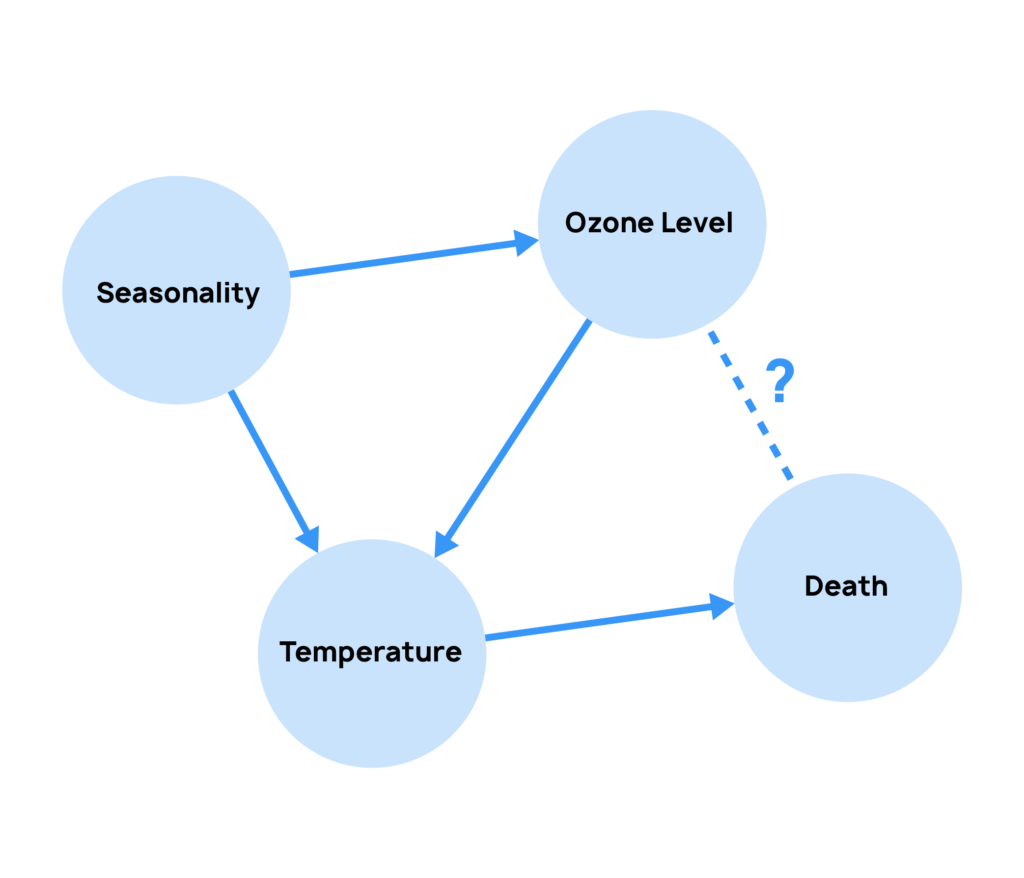
But what is really driving the seasonality? The first suspects are obviously temperature and humidity, which luckily are variables present in this dataset. It’s natural to expect that in colder and rainier weeks, death rates are higher – which also coincides with the peak of incidence of respiratory diseases.
To really assess the causal impact of ozone on deaths, we need to control for the effect of these confounders. In an ideal scenario, we would have two parallel worlds: both with the same temperature, humidity, incidence of flu, demographics… the only difference being the ozone levels. Unfortunately that is still not possible, therefore we need to rely on tools such as causal discovery and causal inference to derive the answer.
Unless we manage to discover all confounding variables, correlations can be misleading as to causation. This is why we need richer datasets, as they have higher chances of containing confounding variables, and robust tools to automatically identify causal relationships from data.
Lag effects
Since we have the variables that explain the seasonal patterns, we can use these to remove the confounding effect of seasonality and look only at the residual relationship between ozone levels and deaths. Effectively, this allows us to synthetically create that control world in which everything else is the same – and we can create a playground where we compare ozone levels with “excess deaths”, compared with the control world. This method is known as a synthetic control and is a very useful way of analyzing causal effects in time-series.
Doing so allows us to ask more meaningful questions: what if there is a time lag between a high-ozone event and a resulting death? To investigate this we can fit a model considering that any of the five days preceding a death may be responsible for it. This reveals that, although the ozone level on the same day with a death did not have an effect, levels aggregated over the previous days do lead to higher deaths.
Correctly factoring in the effects of confounders and temporal patterns is essential if you want to draw causal inferences. Fortunately, we now have a set of formal, mathematical frameworks and powerful tools for making causal claims.
The limitations of conventional tools for causal reasoning
Two of the most prominent formal frameworks for studying causality are:
Granger causality
Granger was a British econometrician and Nobel Prize winner, that gave us one of the first formal definitions of causality: if a signal X1 “Granger-causes” a signal X2, then past values of X1 should contain information that helps predict X2 above and beyond the information contained in past values of X2 alone. However the main limitation of this method is that it fails to capture many important aspects of causality, such as counterfactual dependence. Would X2 still have happened even if X1 had been different? In our example, this method would correctly remove the long-term trend but would fail to discover that temperature was a confounder. Thus, contrary to its name, Granger causality is a method for detecting correlation rather than causation.
Randomized controlled trials
One way of assessing causal relationships in a dataset is to run randomized control trials. In randomized control trials we randomly divide people in two groups, the treatment group, on which we apply an intervention, and the control group, on which no intervention is applied. By comparing the results between the two groups, it’s possible to isolate the effect of the intervention. Thus, this approach avoids the need for counterfactual reasoning, as the control group provides this information.
In many applications, such as marketing, ecommerce and clinical trials, this is feasible – and mostly ethical. But in a time-series setting, running a randomized control trial would imply actually going back in history in order to replicate the world exactly as it was.
This is, of course, impossible. In time-series we are limited by our observations: therefore it’s important to understand how to derive a causal structure from the data – without the ability to intervene in it.
Luckily, causal discovery from observational data – one of the core parts of Causal AI, allows users to – either automatically or with the aid of domain knowledge – go from data to causal graphs. Causal AI can also be used in combination with classical RCTs (see A/B testing with Causal AI) to both help design and optimize experiments, but also to better interpret and analyze results.
Conventional deep learning models are blind to causality
Deep learning models can play board games, drive, make phone calls, even design furniture. But do these machine learning models see the world in the same causal way that we, their users, see it?
We have strong grounds to believe that this is not the case. Take for example this agent playing the Atari game called Pong. The agent, called AlphaGo, is better than humans. It can create tunnels that quickly deplete the tiles, a strategy very similar to the one used by us. But the same agent completely fails when we move its paddle slightly up and to the right. This means that AlphaGo had not understood the physics of the game. Or consider personal assistants like Siri, that use Natural Language Processing models, to understand and analyze our speech. For Siri, asking for “a liter of books” is not unreasonable, because shopping items are often in liters.
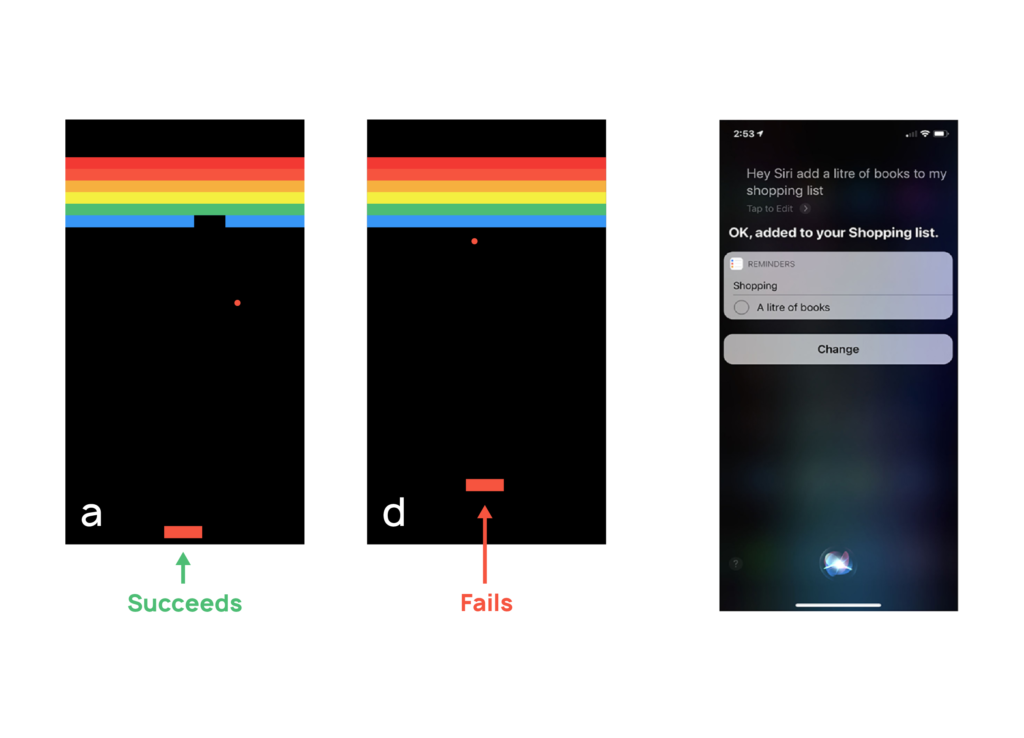
The underlying weakness of these models is that they are blind to the mechanisms determining how their world operates. They simply act based on correlations and if those change, in ways that to us humans seem straightforward, they fail. As in our simple correlation-based model that proposed increasing ozone levels to decrease deaths, these models fail to correctly model the effect of interventions and can prove misleading when advising human policies.
Why Causal AI is the only way
Causal AI is more than a mere application of conventional machine learning models to causal questions—it is a complete reconceptualization of machine learning based on causal mechanisms. Causal knowledge is used to anticipate the impact our actions will have on the environment in question, and thereby formulate plans and strategies accordingly, allowing you to move beyond predictive modeling. For instance, rather than asking “What is the ozone level going to be tomorrow?”, you can instead consider “How would reducing inner city traffic impact ozone levels?”. These types of questions are really important for organizations, because they allow them to understand the implications of actions which they can take within the business environment.
We depend on causal reasoning to imagine possible worlds that differ from our own, a competence that allows us to diagnose why something happened as it did.
Here are two examples of tools with the Causal AI ecosystem:
Causal Graphs
To go beyond the limitations of Granger causality we need tools that clearly capture the interactions between different variables. Causal graphs, popularized by Judea Pearl, are an example of such a tool:they map all the different causal pathways to an outcome of interest and show how different variables relate to each other. In our study of the London Dataset, a causal graph can show that some deaths are caused directly by high ozone levels, while others are caused by low temperatures, which also relate to lower ozone levels.
Causal graphs can either be constructed by domain experts, discovered using causal discovery from observational data, or constructed using a combination of human knowledge and algorithms using Human Guided Causal Discovery approaches.
Structural Causal Models (SCMs)
SCMs are a powerful tool for understanding the causal relationships between variables in a system. An SCM is composed of a set of variables, with some being exogenous and others being endogenous.
The key advantage of an SCM over other types of models is that it explicitly models the underlying mechanisms that generate the data, rather than just the statistical relationships. This allows for a more detailed understanding of the system and the ability to make counterfactual predictions about what would happen if certain variables were changed. SCMs are widely used across multiple fields such as economics, epidemiology, engineering, and computer science. They can be applied to both observational and experimental data, and are a powerful tool for understanding cause-and-effect relationships in complex systems.
Beyond predictions: decisions are objective
It’s not only important to predict deaths, we also need to understand how to reduce them. Knowledge of the causal structure in this problem allows us to ask counterfactual questions: “what would happen if ozone levels were to drop by X%?”, thus paving the way for optimal data driven decisions.
To put it simply, if someone told you in sincerity that rain is less likely if you leave your umbrella at home, you’d question their smarts. And yet this is precisely what a machine learning model without causal knowledge would predict. Conversely, Causal AI allows researchers and practitioners to identify the underlying causes of a particular outcome, and to test interventions that are designed to alter those causes. This allows for the development of more effective and efficient AI systems that can make better predictions, make more informed decisions, and take more effective actions.
Causal AI is the only way to understand and successfully intervene in the world of cause and effect.