- Blog
How to Understand the World of Causality


Introduction
The world of causality is broadly split into two main domains:
- Mainland of causal inference: Causal inference is concerned with understanding the effect of the actions you take. Causal inference provides tools which allow you to isolate and calculate the effect of a change within a system- even if that change never happened in practice. Causal inference can be used to answer the following questions: Did I get better because I took a certain medicine? How much do I have to increase my advertising spend to achieve my revenue targets? What is the effect of classroom size on educational achievement?
- Island of causal discovery: Causal discovery methods take data and determine the cause and effect relationships within it. Crucially, the relationships which causal discovery uncovers are not simply statistical correlations. A causal relationship is invariant to change and represents a more fundamental basis from which to understand a system.
Mountains of Experimentation
The most obvious place to start with the world of causality is with the Mountains of Experimentation. The mountains loom large over the landscape and for good reason. These include the gold standard methods for understanding causal effects with the greatest certainty.
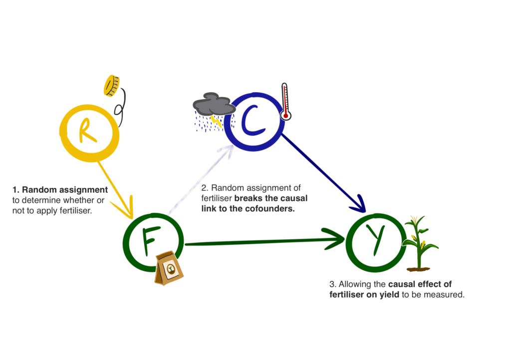
The key to understanding the effectiveness of these methods is by grasping the significance of random assignment. By intervening in the world, experiments randomize those who receive a certain treatment, and those who do not- the control. The treatment could be any number of things: a dose of a drug, an amount of fertilizer applied to a crop, a morning routine.
Since the treatment is randomized, if you select a large enough sample from the population, then statistically speaking the only difference between your treatment and control groups is the treatment itself. You have managed to eliminate all other factors which would normally bias your results. These external factors which have both a causal relationship with your treatment and your outcome are called confounders. All of the causal inference techniques you will read about in this post have the goal of eliminating confounders. Therefore, meaning any difference between the treatment and control groups has to be due to the treatment- thus allowing you to calculate the treatment effect.
Consider the example where you are a farmer and would like to understand the effect of treating your crop with a snazzy new fertilizer. Instead of naively applying the fertilizer to the entire field you could divide the field into squares. For each square you flip a coin and based upon the outcome either apply fertilizer or not. In doing so you have randomized whether or not you apply fertilizer and therefore removed any factors which may bias your choice. Additionally, since you are working within the same field, confounders such as the weather are controlled for and cannot bias the results. You can then simply compare the crop yield of treated squares to those which are untreated gaining you the treatment effect.
City of Natural Experiments
In many cases running a real world experiment is simply not feasible. Experiments can be unethical, prohibitively expensive, logistically impossible, or any combination of these factors. So, what can you do if you are faced with a situation where you cannot run an experiment?
Scientists from a variety of fields have been faced with these situations for generations. Economists cannot scale controlled experiments to the size of nations. Biologists cannot intervene to assign treatments to patients which they suspect to be harmful. Thus, these scientists have developed a host of techniques to identify natural randomization allowing them to remove bias and identify treatment effects without directly intervening themselves. These are the techniques which populate the City of Natural Experiments.
All of the techniques in the City behave in a similar fashion, exploiting natural randomization to calculate treatment effects, but to understand this more deeply it is time to focus on one: instrumental variables. These are variables which do not cause or correlate to the outcome, nor any of the other confounders, but they have a direct causal impact on the treatment. In the graphical form an instrumental variable looks identical to the farmer’s coin flips from the previous section.
Let’s return to our farming example. The farmer’s crop of choice is corn and they would like to understand how much changing the price would impact the amount they sell. The farmer knows that there are a variety of factors which impact their corn sales: cost of transportation, overall yield that year, consumer trends etc. However, our farmer understands that in years with less rain yields are lower, and when yields are lower farmers increase prices.
Now for the weather to be a good instrumental variable our farmer is assuming that:
- The weather and corn sales are not confounded by another factor; one which causes both of them.
- The weather has no effect on corn sales.
If these assumptions are correct, and the farmer’s domain expertise about the corn market also holds that the randomization introduced by the weather, and a large enough dataset, would allow the farmer to calculate the impact of price on corn sales- all without running a real world experiment!
Causal Graph Bridge
Causal inference can be thought as a two stage process: identification and estimation. Identification is the process of determining the set of variables you would need to control for, i.e. hold constant, to isolate the causal effect of interest. Estimation is then the application of statistical techniques to your data to calculate the effect. Causal graphs are the de-facto tool for performing identification.
Causal graphs visualize the cause and effect relationships within the data you wish to explore. You have already seen a causal graph in the preceding section when considering how fertilizer would impact the farmer’s crop yield.
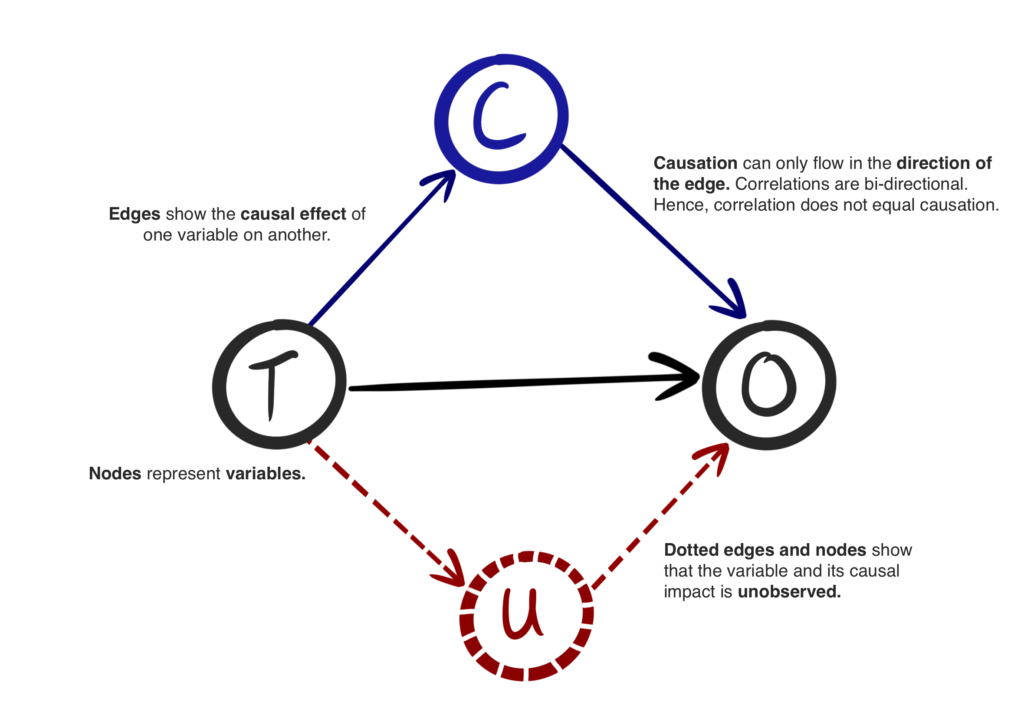
Causal graphs are directed acyclic graphs (DAGs) meaning they represent variables as nodes, with the directed edges between the nodes showing the causal effect of one variable on another. Edges also represent the two-way correlation between variables, while causality is only one way, correlations or statistical associations are two ways. Therefore, correlations can be indicative of causal relationships but are not proof.
One way of thinking about a causal graph is as an estimation into how data is generated. The cause and effect relationships describe how one feature on its own, or in combination with others, results in another- eventually leading to the creation of the feature which you wish to study.
In previous sections you learnt about how randomization can remove the biasing effects of confounding variables. Causal graphs allow you to achieve the same goal, without randomization. This means you do not necessarily need to perform an experiment, or identify a natural source of randomness, to untangle the causal threads within your data.
Causal Discovery Island
Causal discovery is the process of combining algorithms and domain expertise to find an appropriate causal graph.
However, the island of causal discovery is a hard place to live. You are attempting to estimate a causal graph representing a data generating process which you will never observe fully in reality- there is no ground truth. Therefore, with most real world data, causal graphs are best estimates of the data generating process and cannot be verified as true representations of the phenomena at play.
This does not mean that the causal graphs recovered from causal discovery, and which underpin most causal inference, are useless. Far from it- these graphs provide a powerful advancement on the purely statistical methods of machine learning, moving you further towards a mechanistic understanding of your system of interest.
There are a number of different algorithms which you can apply to collected data in order to surface causal relationships. The two most common categories of causal discovery algorithm are:
- Constraint-based: By performing conditional independence tests, where different variables within the dataset are controlled for and the impact of doing so on the other variables is measured, the algorithm can identify certain causal patterns. Applying the conditional independence tests iteratively across the entirety of the dataset then allows a more complete picture of the underlying causal graph to be built.
- Score-based: This class of algorithms proposes a range of different causal structures which are then assigned a score based upon how well they fit with the underlying data. The algorithm starts with basic structures, and then builds upon the best-fitting ones through repeated rounds of scoring to result in a causal structure which encompasses the available variables.
The catch with applying algorithms to your data is that they can never retrieve a fully resolved causal graph. The output will always have some edges which do not have a clear causal direction, and this is where human domain knowledge comes in. Domain expertise is crucial in creating a usable causal graph, and is therefore critical in obtaining accurate causal discovery results.
The final hurdle with causal discovery is the presence of unobserved confounders. These are variables which confound your variables of interest, but are not present in your dataset. Without observation these confounders mean that many causal inference methods do not work. Causal discovery methods, and human domain expertise, can be powerful here as they can help to flag where unobserved confounders may be influencing the data generating process.
Matching Forest
The Matching Forest is where Causal Graph Bridge makes landfall. Causal graphs allow you to easily understand which variables to control for when attempting to estimate a causal effect. The techniques within the Matching Forest provide you with the tools to move from the graphical world to application within your data. Matching techniques are well understood and widely used within the literature- leading to a lush green forest.
Matching is the process of removing confounding effects between a treatment and an outcome by constructing comparison groups that are similar according to a set of matching variables. Those matching variables are typically identified using your causal graph.
The intuition here is that you are constructing a control group which has similar properties to your treated group. Therefore any variation in outcome between the two must be due to the treatment, leading to an estimate of the causal effect.
The simplest matching tool is subclassification.
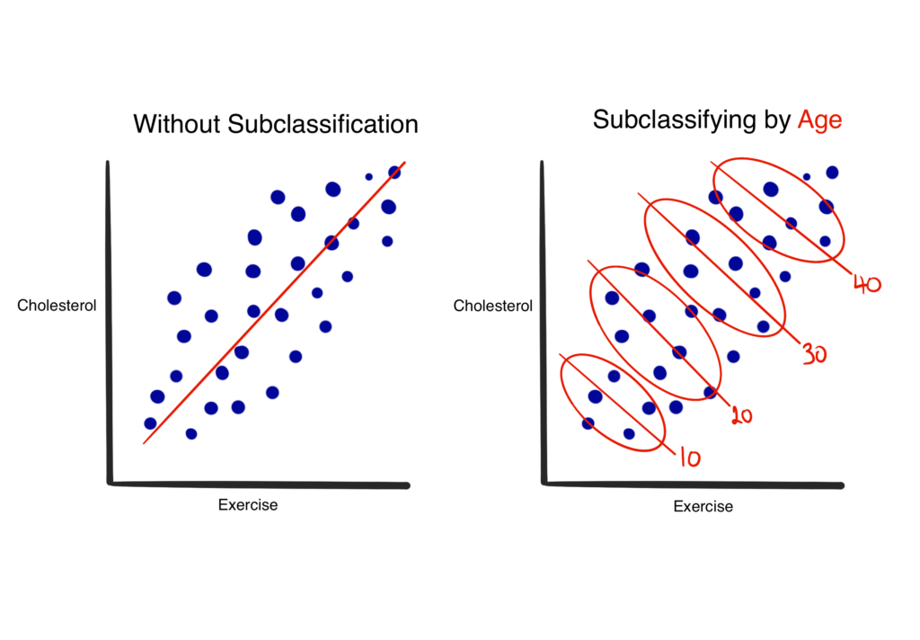
When plotting the treatment (exercise) against the outcome (cholesterol) data you notice a downward trend, as in the left hand side of the figure above. However, by bucketing the data by the confounding variable (age), therefore creating subclasses, you can then observe the true relationship between your treatment and outcome- see the right. Subclassification is intuitive and easy to grasp, however as the number of variables you need to control for grows the amount of data required skyrockets. This limits the applicability of subclassification in many cases, leading to the other methods which populate the Matching Forest.
Modeling Swamp
The Modeling Swamp is where things begin to get a little murky. The modeling swamp is home to some of the most familiar causal inference tools, in contrast with less established newcomers. Models provide powerful methods for estimating causal effects, and while some rely on a fully specified causal graph, others can act effectively without that requirement.
The most popular method within the modeling swamp is plain old regression. Ordinary least squares (OLS) regression is a massively flexible and valuable tool for the estimation of causal effects. It is popular for good reason too:
- Theoretically well understood: OLS and other types of regression methods are very well understood from a statistical point of view. This means that the assumptions of applying regression to your challenge are clear, allowing you to make informed choices about the results.
- Interpretable: Regression models are readily explained, unlike more modern machine learning techniques. This makes them great for use in higher stakes cases, such as when regulation is involved.
- Causal Inference is Simple: Controlling for confounders and estimating causal effects using regression is straightforward. The learned coefficients within the regression equation are the estimates of the causal effect of a given variable, while controlling for the others- see the figure below.

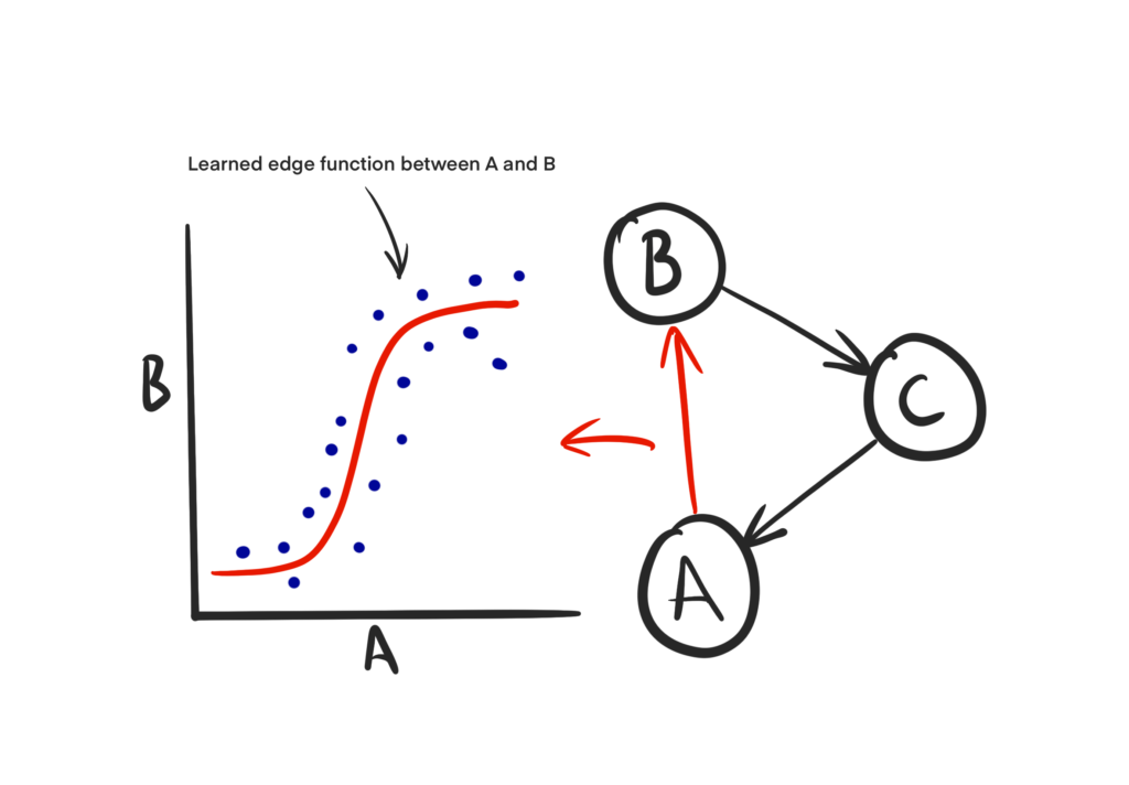
The second method here which is worth understanding in more detail is the structural causal model (SCM). The SCM builds directly from the foundations of the causal graph and learns the mathematical forms of the causal relationships identified by domain expertise or algorithmic causal discovery.
This means that the edges and nodes within your causal graph now have mathematical relationships learnt from the data. This is incredibly powerful as it allows you to easily create “what-if” scenarios by intervening in the model. Intervening simply means changing the value of a node within the graph. The SCM then describes how this change would flow through to the other variables, and eventually the treatment. The result is that with a representative SCM you can begin to explore a huge range of different scenarios, and compare the impact of different actions.
Decision Intelligence Desert
The Decision Intelligence Desert is barren and remote, however there are oases. This area of the map encompasses the burgeoning number of techniques which go beyond treatment effect estimation. To provide an illustration of the types of methods contained with the desert let’s consider algorithmic recourse.
In machine learning a common type of explainability technique are counterfactual explanations. Counterfactual explanations pose the question; what would have had to be changed in order for the outcome to be different?
For example, imagine a retention machine learning model which has predicted that a customer will churn. A counterfactual explanation to help explain why this person is likely churn could be: if they were a senior customer aged 65 or over, they would renew.
Algorithmic recourse builds from the notion of counterfactual explanations but with a focus on providing you with the ability to act, rather than simply understand. Therefore, algorithmic recourse provides the ability to recommend actions in order to change unfavorable outcomes, allowing you to intervene in the system to prevent them.
This ultimately changes the churn example above from an unactionable explanation, to an actionable recommendation. Applying recourse to prevent this person from churning: if they received a 10% discount, they would renew. As discounts are something which can be acted upon this allows you to affect change in the real world.
Conclusion
You have been on a whirlwind tour of what is a deep and fascinating subject. I hope that you have enjoyed your adventure into the world of causality, and that you feel motivated to learn more.
If you do wish to dive deeper I would highly recommend the following books and resources as a jumping off point:
- Brady Neal’s Causal Inference course on Youtube: A great introductory video series which will bring you up to speed with many of the topics discussed in this post.
- The Effect, or Causal Inference the Mixtape: Books focusing more on the traditional techniques of causal inference. These will provide you with a powerful foundation to continue your journey. Both books are kindly made available for free by their authors, but I would always recommend getting a physical copy if you can afford it!
- Causal Inference for the Brave and True: A really interesting read into how the worlds of causal inference and machine learning are colliding. Has great hands-on code samples which allow you to learn practically!